AWS Storage Blog
Inside the AWS Storage Assessment: How intelligent analysis replaces guesswork
A completed storage assessment looks simple: an AWS Storage service recommended per workload, capacity and performance recommendations, and cost. This post walks through the analysis of how we go from analyzed data to right-sizing on AWS.
In Part 1 of this series, we covered what an AWS Storage Assessment delivers: service recommendations, right-sized configurations, and validated cost models from actual telemetry. Teams planning storage migration need this because manual estimates miss workload characteristics that drive cost and architecture decisions. A single RVTools export or a 30-day NetApp Data Infrastructure Insights collection produces a per-workload business case ready for leadership review.
The numbers in an assessment (68% of capacity inactive, high-confidence classification, 60–80% cost reduction from I/O density tiering) are not spreadsheet formulas. They come from a multi-stage pipeline of detection, classification, and optimization that weighs many dimensions at one time, whatever the source. Understanding it helps you judge an assessment before acting on it.This post covers six stages:
- Automatic workload classification.
- Inactive data and infrastructure detection.
- Right-sizing and efficiency modeling.
- Configuration optimization.
- Data protection cost modeling.
- Scenario analysis with what-if engine.
Automatic workload classification
Most storage assessments require a storage architect to manually tag every volume by workload type. For 1,000 volumes across multiple arrays, this takes days and introduces errors that compound through the analysis, for example, a backup server sized as a file server, or a database volume priced as archive. The assessment instead runs an automated classification pipeline that adapts to whatever data source you provide.
Classification adapts to source quality
Different data sources carry different signals, and the assessment adapts to each. Rich performance-telemetry sources (NetApp Data Infrastructure Insights, Dell InsightIQ) let it classify by what a volume is, from array metadata such as protocol, IOPS patterns, and share associations. Hypervisor exports (RVTools, vSphere) and discovery tools (AWS Transform, ModelizeIT, Cloudamize) let it classify by what a server does, from naming patterns, application detection, and measured IOPS. Manual templates provide user-declared mappings, validated against protocol and capacity signals.
The classification pipeline
For sources requiring inference, each volume passes through four stages in priority order, as detailed in the following table.
| Stage | What it evaluates | Example |
| Keyword matching | Server names, volume names against known function tokens | SQLSRV01 matches “SQL,” classifies as database. BKPSERVER matches “BKP,” classifies as backup |
| Segment-aware parsing | Structured decomposition of concatenated enterprise identifiers | DSSPTVBP040 decomposes to site (DSS) + platform (PTV) + function (BP) + sequence (040). Backup detected at position 6. |
| Protocol corroboration | NFS/SMB/iSCSI from storage config narrows service candidates | NFS + file server name tokens = high-confidence file server |
| IOPS behavior | Peak IOPS density compared to workload profiles | 50 TB at 200 IOPS (0.004 IOPS/GB) = cold regardless of name |
The stages run in priority order, and the parser uses word-boundary awareness to prevent false positives (for example, “Profiles-1” does not match “FILES”). Each classification carries a confidence score. Where multiple signals agree, the volume classifies automatically; where they conflict or fall below the threshold, it’s flagged for human review rather than guessed.
Infrastructure separation
Before sizing runs, the assessment identifies infrastructure components that would distort results if treated as customer workloads:
- VMware vCLS agents, Nutanix Controller VMs, hypervisor appliances, VM templates
- Powered-off servers (not consuming IOPS, excluded from performance sizing)
- Desktop operating service instances (outside storage scope)
- Storage constructs: clone volumes (full-capacity sizing double-counts shared blocks), datastore-backing volumes (already counted using their VMs), replication destinations (treated separately), distributed volume fragments (parts of a scale-out file system; the parent is the real workload), and tiering targets (cold data already counted in the source volume)
All exclusion decisions are surfaced with volume counts and capacity attribution. The assessment identifies candidates; the customer confirms.
From classification to service routing
Classification then drives service routing, shown in the figure 1.
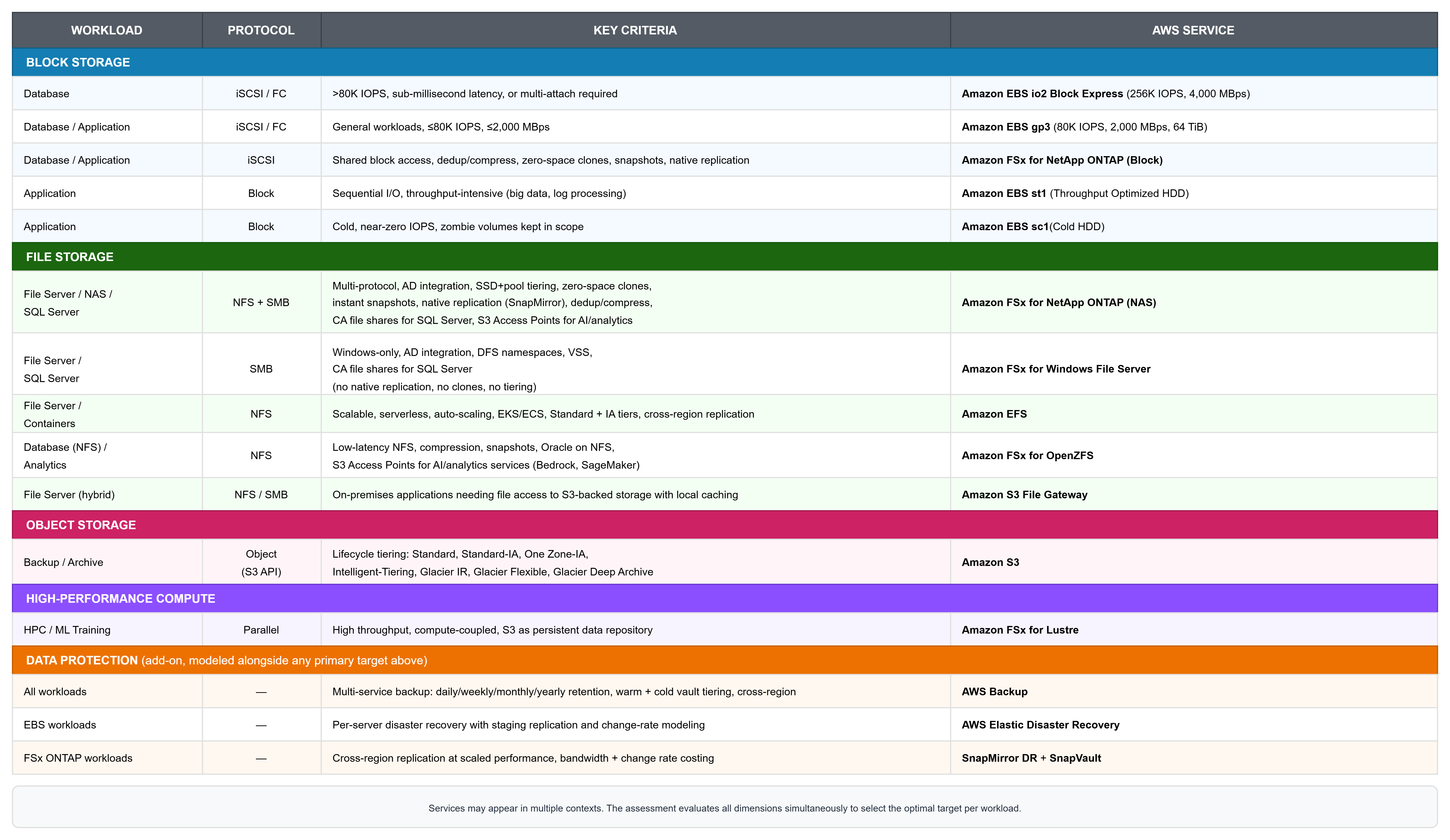
Figure 1: Service routing: How AWS Storage Assessments map workload characteristics to AWS storage services
The key components are routed as follows:
- Database and application servers – Route to Amazon Elastic Block Store (Amazon EBS) (gp3, io2 Block Express, st1, sc1) or Amazon FSx for NetApp ONTAP block based on protocol, peak IOPS, latency sensitivity, and sequential versus random I/O patterns.
- File services – Route to FSx for ONTAP (including NetApp FlexCache for multi-Region read caching), Amazon FSx for Windows File Server, Amazon Elastic File System (Amazon EFS), Amazon FSx for OpenZFS, Amazon S3 Files, or Amazon S3 File Gateway based on protocol (NFS or SMB), combined group capacity, throughput requirements, access patterns, and hybrid access needs. Groups above a consolidation threshold route to shared file services where multi-tenant efficiency reduces cost.
- Backup repositories – Route to Amazon Simple Storage Service (Amazon S3) with lifecycle tiering across storage classes (Standard, Standard-IA, One Zone-IA, Intelligent-Tiering, Glacier Instant Retrieval, Glacier Flexible Retrieval, Glacier Deep Archive) based on sequential I/O patterns, large capacity, and low IOPS density.
- Archive and inactive volumes – Route to S3 Glacier storage classes (Instant Retrieval, Flexible Retrieval, Deep Archive) based on infrequent access patterns.
- High-performance parallel workloads – Route to Amazon FSx for Lustre based on high throughput density and compute-coupled access patterns.
- Mixed environments with NAS, block, and object workloads – Split automatically and route to multiple services in parallel.
Rather than just a label, the output is a service mapping, target configuration family, and confidence score, ready for the sizing engine.
Inactive data and infrastructure detection
After every workload is classified, the next question is how much of it should move at all. One of the highest-value findings is data that consumes expensive primary storage but serves no active workload. In the NAS example from Part 1, 844 of 3,920 volumes (1,720 TB) showed zero I/O activity over a 30-day collection, capacity that can be archived, tiered, or decommissioned before migration to cut both migration scope and ongoing AWS cost.The assessment flags three kinds of non-productive capacity before sizing:
- Zombie volumes – Volumes with zero IOPS and zero throughput over the full collection period (7–30 days). In the environments we assess, a significant share of capacity commonly sits idle. Each is flagged with its capacity so you can archive it to S3 Glacier, decommission it, or keep it in scope; moving inactive data to S3 Glacier Deep Archive can cut its cost by up to 99% without application migration.
- Replica and data-protection copies – Replication destinations duplicate source data, and sizing them alongside primaries can inflate estimates by roughly 30–50%. The assessment identifies them from source metadata and reports them separately so you can exclude them or plan independent migration. In the NAS example from Part 1, 646 replication volumes (646 TB) were identified.
- Duplicate mount paths – NAS environments often expose the same volume across multiple mount paths. Two-pass deduplication (exact path matching, then server and capacity fingerprinting) collapses these.
Net impact
In the environments we assess, these detection stages typically reduce the in-scope workload set by 20–40% before sizing begins (in the VMware example from Part 1: 7,743 VMs reduced to 5,050 in-scope). Volumes removed at this stage are volumes that don’t generate AWS cost in the recommendation.
Right-sizing and efficiency modeling
With inactive data set aside, sizing focuses on what remains. The biggest savings come not from choosing the cheapest service, but from accurately determining how much capacity and performance each workload needs. On-premises storage is almost always over-provisioned, and that gap is budget that does not need to move to AWS.
Three capacity modes
The assessment supports three approaches to capacity sizing:
- Provisioned – Sizes on total allocated capacity. Used when utilization data is unavailable or the customer wants to preserve existing headroom.
- Used + buffer – Sizes on actual consumed capacity plus a configurable buffer. For the NAS example from Part 1 (10,667 TB allocated, 4,817 TB used), this reduces target capacity by 50% before any other optimization.
- Intelligent mode – Applies per-workload logic based on utilization ratio, volume size, and performance characteristics. High-utilization volumes keep provisioned capacity; low-utilization volumes with low IOPS get aggressive right-sizing.
In the environments we assess, switching from provisioned-based to utilization-based sizing typically reduces costs by 40–60%.
Vendor-aware storage efficiency ratio
AWS storage services like FSx for ONTAP provide inline deduplication, compression, and compaction. If the source environment already runs these features (common on NetApp ONTAP, Pure Storage, and other modern arrays), the used capacity already reflects those savings. The assessment applies vendor-aware modeling:
- Data from already-deduplicated sources receives zero additional efficiency credit. Applying an additional deduplication assumption would undersize the target, leading to capacity shortfalls post-migration.
- Data from non-deduplicated sources receives the target service’s expected efficiency ratio, because those savings will genuinely be realized on the target for the first time.
This is the most common error in manual assessments.
I/O density-based data tiering
FSx for ONTAP provides multiple automatic tiering policies that move data between SSD and capacity pool based on access patterns. The assessment determines the optimal policy per volume based on I/O density, as shown in the following Figure 2.
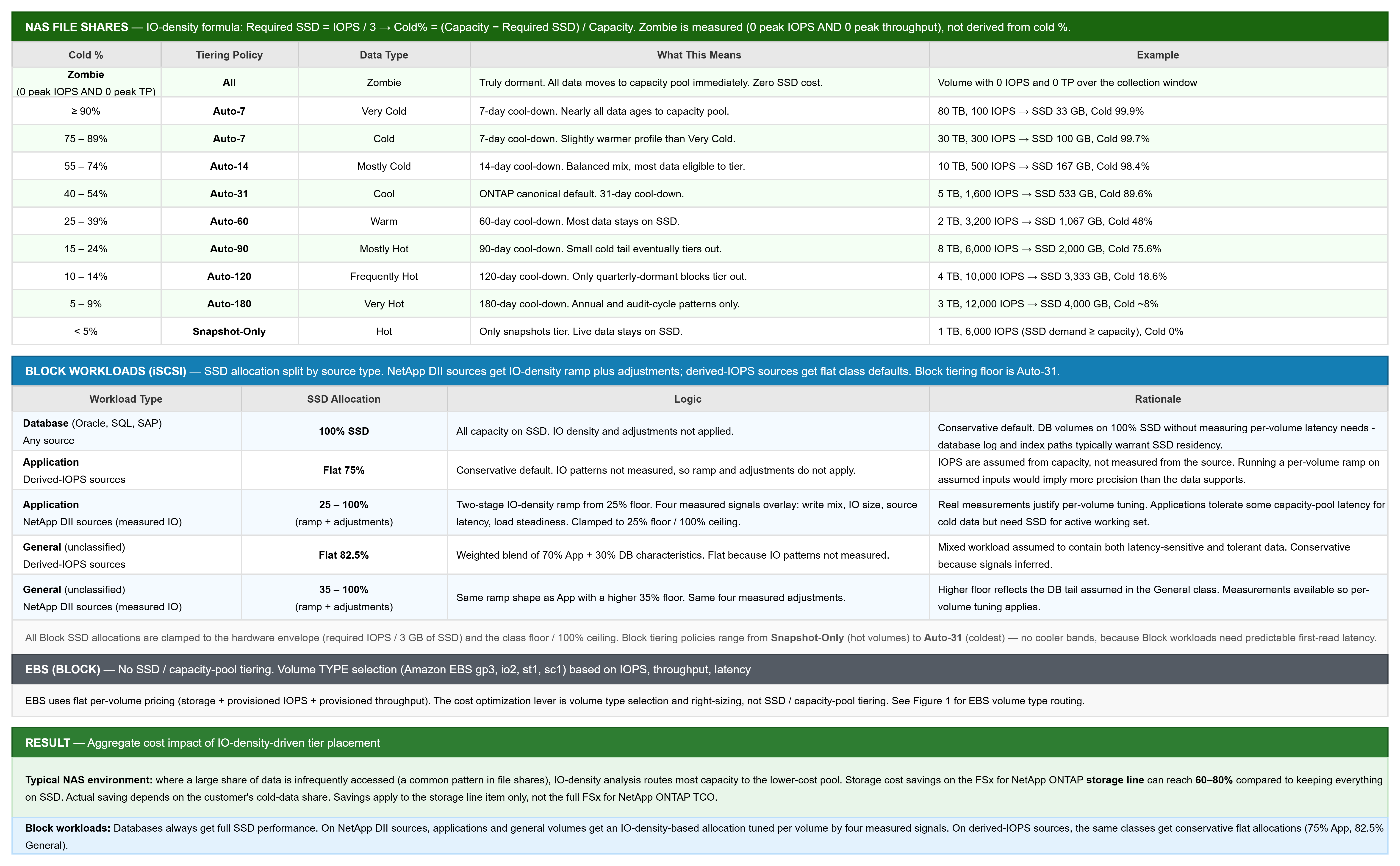
Figure 2: I/O density analysis: How the assessment determines SSD compared to capacity pool allocation
Allocation is set by workload type. For NAS file shares, IO density (IOPS per GB of used capacity) drives the split: busier data stays on SSD, sized to roughly 3 IOPS per GB, and the quieter remainder moves to the lower-cost capacity pool. For block workloads, databases get 100% SSD because they cannot tolerate capacity-pool latency, while application and general workloads get a graduated allocation. On sources with real measured IO patterns, the assessment tunes the SSD share per volume based on the workload’s write mix, IO size, latency, and load steadiness. On sources with derived IOPS (RVTools etc.), a conservative flat allocation is used. Because most NAS data is infrequently accessed, tiering the cold portion can cut storage costs by roughly 60 to 80 percent versus all-SSD.
Peak versus average analysis
Peak versus average analysis Performance sizing uses peak values from the collection period, not averages. For sources with array performance data, per-volume IOPS are scaled against the array’s observed peak rather than summing individual peaks (which would overstate requirements due to non-overlapping peak windows).
Configuration optimization
Right-sizing capacity is necessary but not sufficient. AWS storage services have configuration parameters (throughput tiers, availability options, volume types, deployment generations) that significantly affect both cost and performance. The assessment selects the optimal configuration, not just the service.
Amazon EBS volume type selection
EBS volume type selection (gp3, io2 Block Express, st1, sc1) is driven by IOPS, throughput, latency, capacity, and multi-attach requirements. gp3 handles up to 80,000 IOPS and 2,000 MBps; workloads exceeding these limits or requiring sub-millisecond latency route to io2 Block Express. Sequential workloads route to st1; near-zero activity volumes route to sc1.
Workloads exceeding single-volume limits are automatically split, with separate boot volume costing for virtual servers.
Amazon FSx for NetApp ONTAP configuration
Picking the right FSx for ONTAP configuration is less like choosing a product and more like solving a puzzle with several constraints at the same time. The assessment evaluates a matrix of configurations across throughput tiers, deployment options, and generations. A Gen2 Single-AZ file system scales to 12 HA pairs (up to 6,144 MBps, 200,000 SSD IOPS, and 512 TiB of SSD per HA pair, reaching 72 GBps and 2.4 million IOPS), whereas Gen2 Multi-AZ and Gen1 file systems use a single HA pair (Gen1 up to 192 TiB of SSD per file system). Each configuration has defined limits for IOPS, throughput, and SSD capacity.The optimizer selects the lowest-cost configuration that satisfies every constraint at the same time: aggregate IOPS and throughput (with a headroom buffer), total SSD capacity (hot data plus buffer and snapshot space), SVM count, and per-file system volume limits. When no single file system satisfies all of them, it calculates multi-file system layouts automatically, comparing eight deployment options (Cost Optimized and Performance Optimized, across Single-AZ and Multi-AZ, for Gen1 and Gen2) so you can weigh cost against availability with real numbers. Figure 3 shows how the optimizer searches this space.
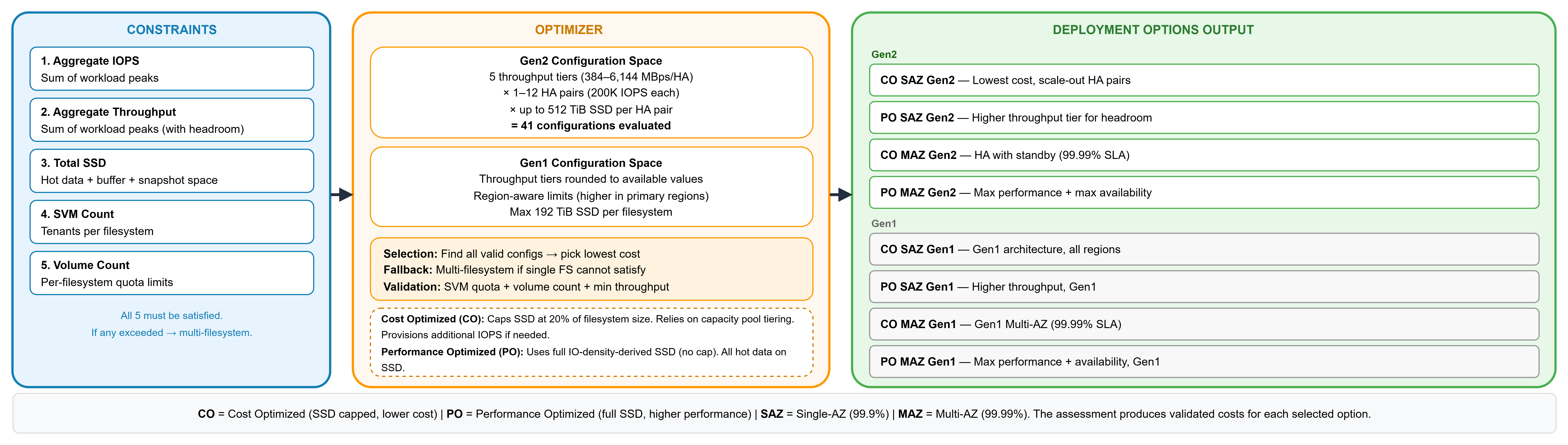
Figure 3: Amazon FSx for NetApp ONTAP configuration optimization: Multi-constraint selection across Gen1 and Gen2
Other service optimizations
You can also consider additional service optimizations:
- Amazon FSx for Windows File Server – SSD versus HDD routing based on latency and IOPS density, with multi-file system splitting when throughput exceeds single-file system limits.
- Amazon EFS – Throughput mode selection (Bursting versus Provisioned) based on peak demand relative to stored-data baseline, with Standard/IA tier split derived from access patterns.
- Amazon FSx for OpenZFS– Multiple architecture options evaluated (Single-AZ, Multi-AZ, Intelligent Tiering to Amazon S3) with 512 TiB capacity enforcement. Compression mode selected per volume, with database data and redo volumes receiving zero compression per AWS best practice.
- Amazon FSx for Lustre – Automatic SSD versus HDD determination with Amazon S3 as persistent data repository.
- Amazon S3 File Gateway – Evaluated for hybrid file access patterns requiring on-premises NFS or SMB access to Amazon S3 backed storage with local caching.
Costs are calculated from the AWS Pricing API for the selected AWS Region at assessment time.
Data protection and cost modeling
Backup and disaster recovery are often left out of a migration estimate, and then get billed for later. The assessment models data protection costs alongside primary storage, so your business case reflects total operational spend, not just storage fees. It models four protection services:
- AWS Backup – Retention across daily, weekly, monthly, and yearly cycles, with warm and cold vault tiering. Rather than estimating backup size as a flat percentage, the model accounts for overlapping retention windows (a single snapshot can satisfy multiple cycles), so the number reflects real backup volume. Cross-Region replication and per-service rates (Amazon EBS, Amazon FSx, Amazon EFS) are priced independently.
- AWS Elastic Disaster Recovery – For Amazon EBS workloads, the model adds per-server staging costs and multiplies by change rate to capture the true cost of ongoing replication.
- NetApp SnapMirror cross-Region replication – The assessment reruns FSx for ONTAP sizing for the disaster recovery Region at scaled performance, then adds transfer costs based on bandwidth and change rate.
- ONTAP SnapVault – Secondary-tier backup, with configurable retention policies and destination throughput-tier selection.
Scenario analysis: The what-if engine
A single recommendation is rarely the end of the conversation. Migration planning means weighing alternatives: different Regions, targets, scope boundaries, and assumptions. Rather than rerunning a full assessment for each, the engine explores five dimensions from one data collection:
- Target comparison – Remap all workloads to a single service and compare costs side by side against the multi-service recommendation
- Region comparison – Re-price the entire workload set across multiple Regions using live pricing, flagging unavailable services
- Scope adjustment – Filter to a workload subset (production-only, specific applications, capacity thresholds) without re-uploading or re-detecting
- Architecture scenarios – Run parallel what-ifs with different deployment options per workload group (for example, Performance Optimized Multi-AZ for production, Cost Optimized Single-AZ for dev/test)
- Parameter sensitivity – Adjust efficiency ratios, growth buffers, or peak percentage assumptions globally and see cost impact instantly
From single collection to decision matrix
Let’s return to the VMware example from Part 1 (5,050 in-scope workloads). Questions like “What if we migrate production only,” “What about eu-west-1 instead of US,” or “Performance Optimized Multi-AZ for production, Cost Optimized Single-AZ for dev and test” each resolve in seconds from the same source data, as Figure 4 shows.
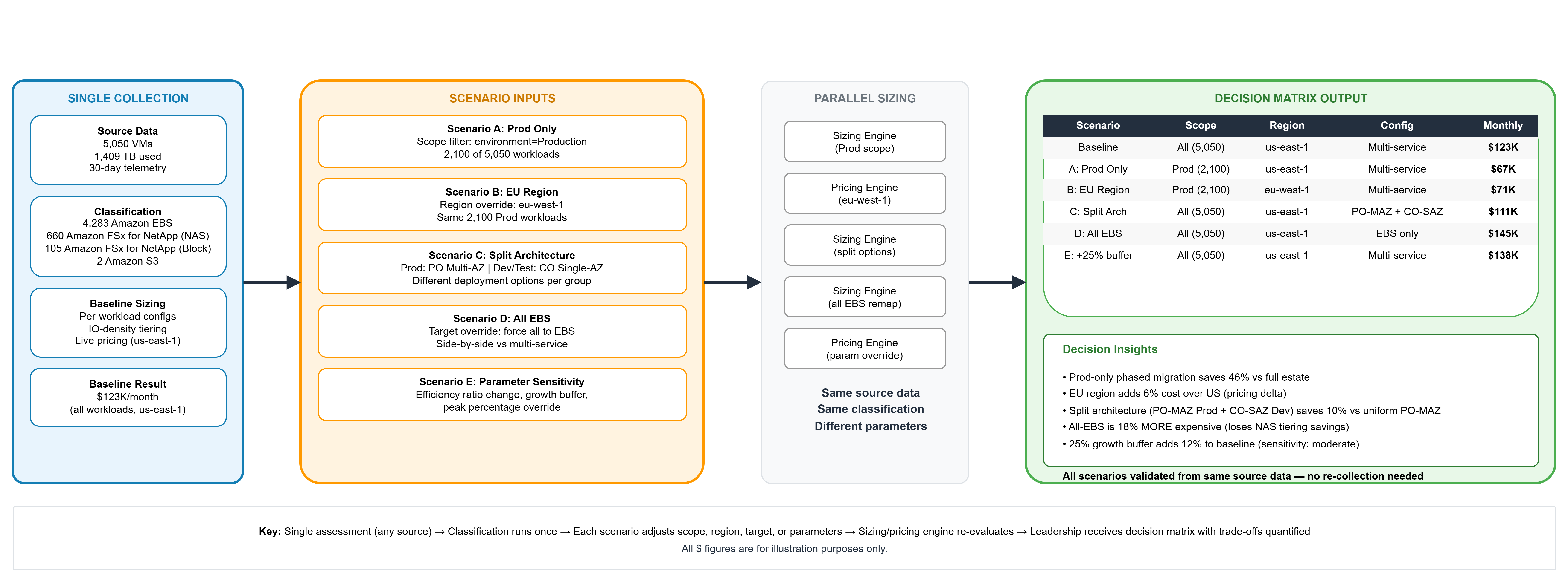
Figure 4: What-if scenario flow: Single data collection, to multiple validated scenarios, to decision matrix
Each scenario uses the same source data. The output is a decision matrix that teams present leadership with trade-offs clearly articulated: cost versus availability, Region versus compliance, phased versus full migration. Rather than a single recommendation, the assessment offers a set of validated options enabling informed decisions.
Conclusion
In this post, we covered the analytical methods that separate a data-driven assessment from a spreadsheet estimate: automated classification, inactive data detection, vendor-aware efficiency modeling, I/O density tiering, multi-constraint configuration optimization, and scenario analysis. Each stage removes a source of error that manual methods leave in place. The techniques apply regardless of source type, and the results are validated against live AWS pricing.
Contact your AWS account team, email migration-assessment@amazon.com, or request an assessment. AWS Migration Solutions Architects run these end-to-end scenarios collaboratively with the customer at no cost. For self-service analysis, AWS Transform assessments provides automated storage assessment capabilities that process telemetry data from multiple sources.
For the full process and examples, see Data-driven planning for cloud migration using AWS Storage Assessment.
Learn More
Read part 3 of this blog series: Planning data protection before migration: How AWS Storage Assessments model backup and disaster recovery costs